Pan Sharpen Landsat Imagery in QGIS

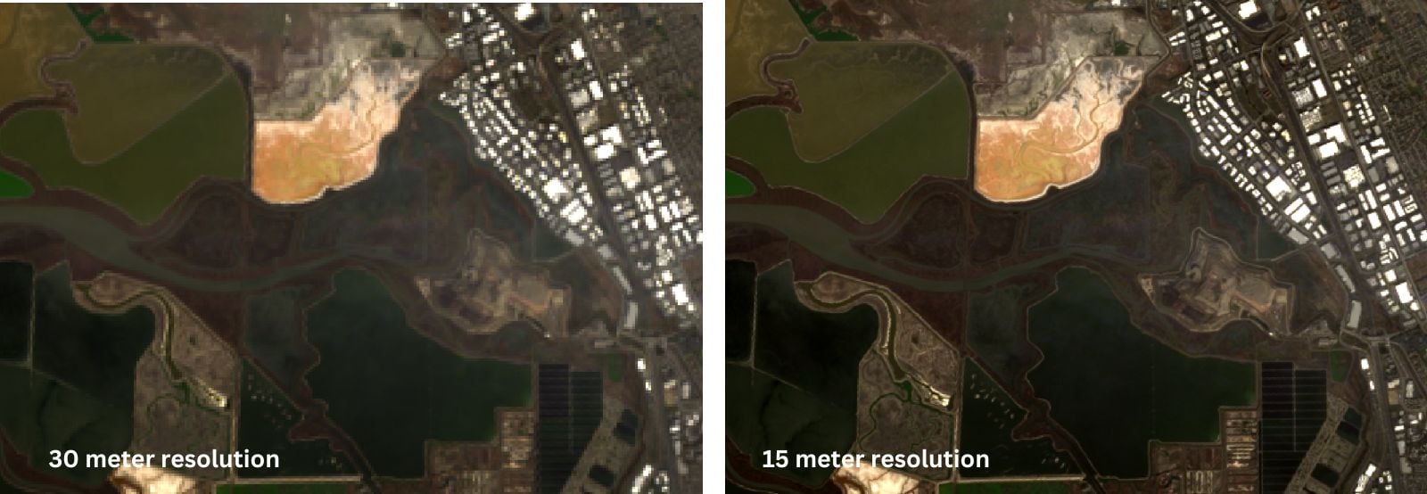
Pan sharpening is a widely used technique to enhance the spatial resolution of multispectral satellite imagery. This process combines the high-resolution panchromatic band of a satellite image with its lower-resolution multispectral bands, producing a visually detailed image without losing color information.

For Landsat imagery, pan sharpening is particularly useful since its panchromatic band (Band 8) has a resolution of 15 meters compared to the 30-meter resolution of the multispectral bands. This article provides a step-by-step guide to pan sharpening Landsat imagery using QGIS, an open-source geographic information system.

Why pan sharpening is important

Landsat imagery is commonly used for environmental monitoring, urban planning, and agricultural analysis. However, the 30-meter resolution of the multispectral bands can limit detailed observations. By integrating the higher resolution of the panchromatic band with multispectral data, pan sharpening improves the visual interpretability of the imagery, making it easier to identify features such as roads, buildings, and vegetation patterns.

Pan sharpening using QGIS is one way to upscale natural color Landsat imagery from 30 to 15 meter resolution using the panchromatic band. The first step is to find Landsat imagery and download the appropriate bands.

Accessing Landsat imagery for pan sharpening

The USGS makes Landsat imagery products freely available via EarthExplorer. EarthExplorer is a free online platform for accessing geospatial data, including satellite imagery, aerial photographs, and digital elevation models. It provides an extensive archive of datasets, such as Landsat, Sentinel-2, MODIS, and radar data, with tools for searching by location, date, and data type. 

While users can browse and search for data, an EROS registration (free) is required in order to download data from EarthExplorer. Once you have set up your login, you can then search by text or via the map interface for an area of interest.

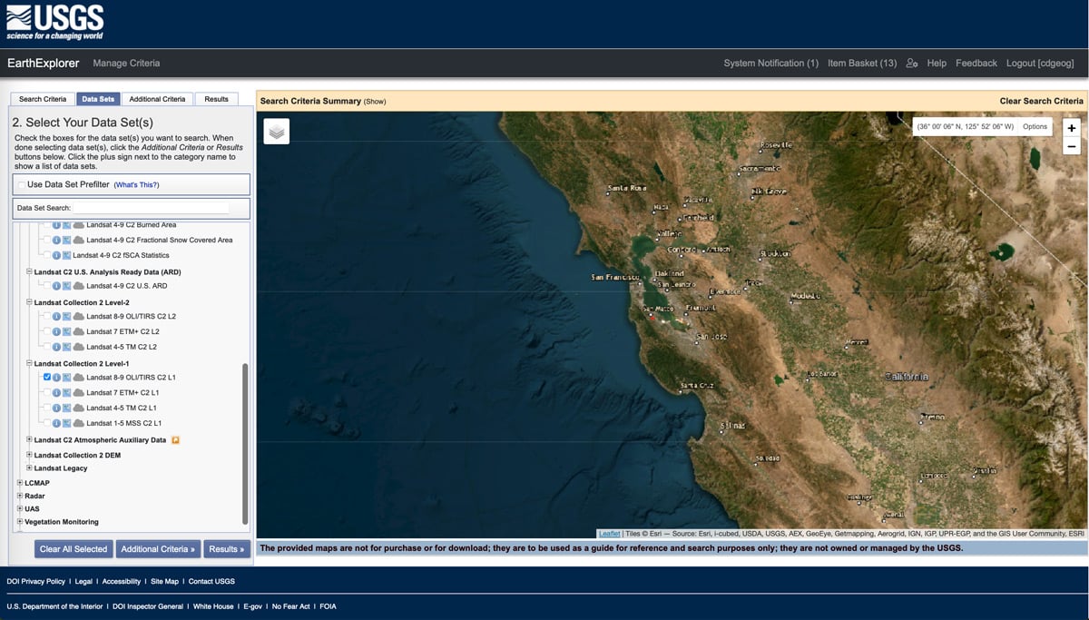
This tutorial uses Landsat imagery of the San Francisco Bay Area. Once the area of interest has been set under the Search Criteria tab, navigate to the Data Sets tab to select the Landsat data product. This tutorial uses the RGB and panchromatic bands from Landsat 8/9 data. To search for those, click on the plus symbol next to the Landsat Collect 2 Level-1 menu option and then select Landsat 8-9 OLI TRIS C2 L1.

Then click on the Results button at the bottom of the page. This will return a list of Landsat images that overlap with the geographic area of interest. In the results pane, find an image tile that you want to use and then click on the download option icon (fifth icon in the list).

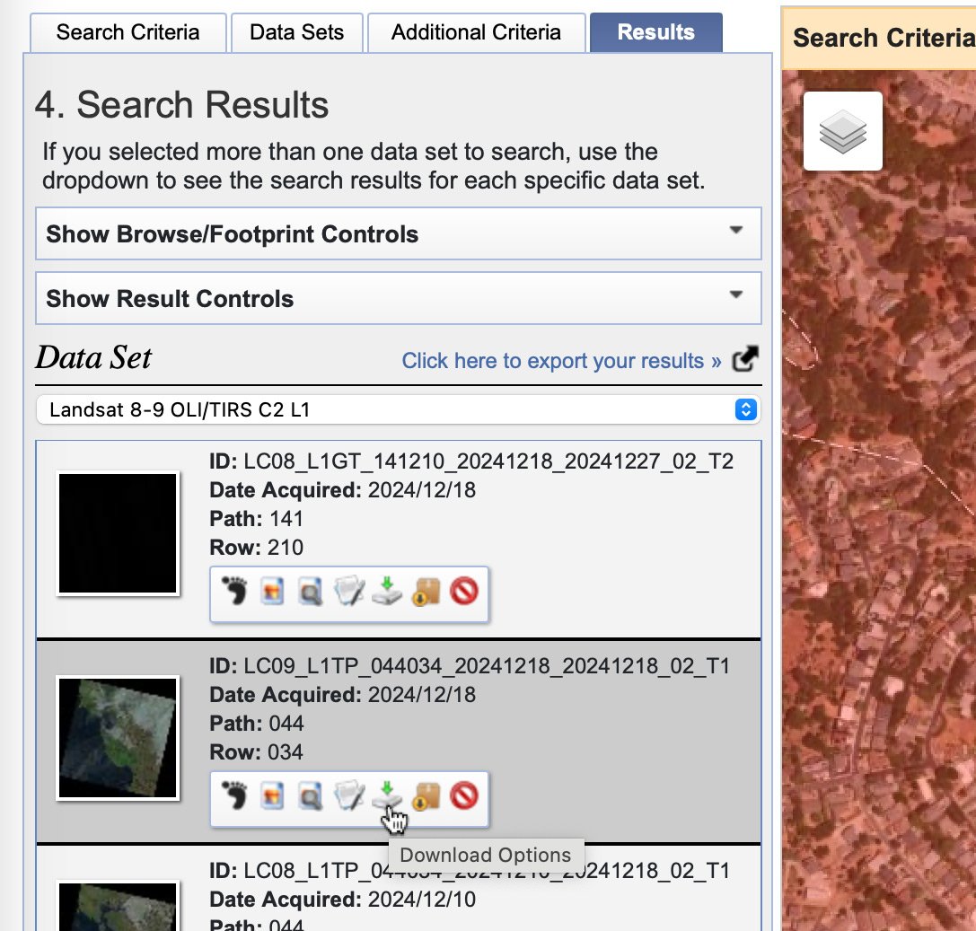
Next click on the green button that says “Select Files”.

Selecting the Landsat spectral bands

Landsat 8 and 9, with the Operational Land Imager (OLI) and Thermal Infrared Sensor (TIRS), capture data across 11 spectral bands, including visible, NIR, SWIR, and TIR wavelengths. 

There are nine spectral bands from OLI:

• Band 1 Coastal Aerosol (0.43 – 0.45 µm) 30 m
• Band 2 Blue (0.450 – 0.51 µm) 30 m
• Band 3 Green (0.53 – 0.59 µm) 30 m
• Band 4 Red (0.64 – 0.67 µm) 30 m
• Band 5 Near-Infrared (0.85 – 0.88 µm) 30 m
• Band 6 SWIR 1(1.57 – 1.65 µm) 30 m
• Band 7 SWIR 2 (2.11 – 2.29 µm) 30 m
• Band 8 Panchromatic (PAN) (0.50 – 0.68 µm) 15 m
• Band 9 Cirrus (1.36 – 1.38 µm) 30 m

For this tutorial, we are interested in Bands 2, 3, 4, and 8.

In the Related Files interface, click on the “Deselect All” link. Then toggle back on B2.TIF, B3.TIF, B4.TIF, and B8.TIF. This selects the the Blue, Green, Red, and Panchromatic bands.

Next click the green “Download All Selected Now” button at the bottom to store the Landsat imagery on your computer.

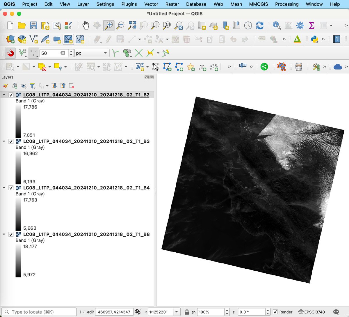
Adding Landsat spectral bands to QGIS

Next open up QGIS. Navigate to the folder on your computer where the four Landsat imagery TIFs are stored. You can simply drag and drop the files into QGIS to display them.

If you haven’t already done so, change the CRS to the correct UTM zone for your Landsat imagery by going to Project –> Properties –> CRS from the top menu item. (Northern California is part of Zone 10 for this tutorial).

Merge the color bands into one image

All of the bands by default display with a gray gradient. The next step is to merge the Blue, Green, and Red bands into one natural color satellite image.

To do this, select from the top menu: Raster –> Miscellaneous –> Build Virtual Raster. In the interface, select the three dots to the right of the Input Layers box (1) and select the three files for Bands 2, 3, and 4. Next, select the location on your computer to store the VRT file (2). Finally, make sure the “Place each input file into a separate band” is selected.

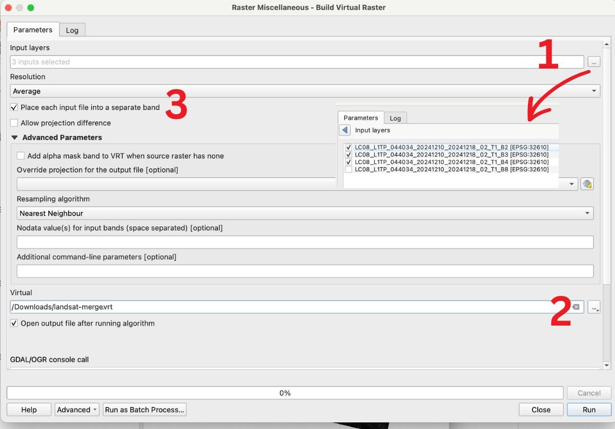
Once all the parameters are set, click on the Run button.

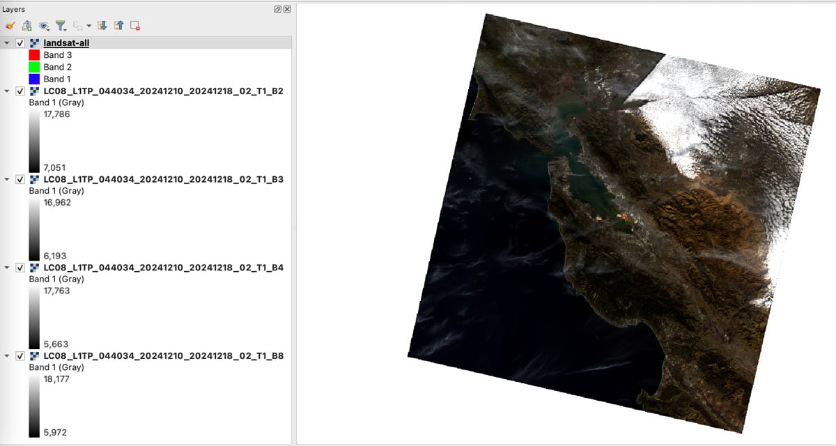
A merged natural color satellite imagery will then be added to QGIS. Make sure the bands in the legend are listed in the order of Blue (Band 1 in the legend), Green (Band 2 in the legend), and Red (Band 3 in the legend) to match the Landsat spectral band order. Otherwise your image will not look natural.

Pan sharpening the Landsat image

Now that the Blue, Green, and Red bands have been merged into one image, we can increase the 30 meter resolution of the multispectral image to match the 15 meter panchromatic band.

Add the Processing Toolbox to a pane in QGIS by going to View –> Panels –> Processing Toolbox. A new panel to the right of the map canvas will load. In the suite of GDAL tools under Raster Miscellaneous select the Pansharpening tool.

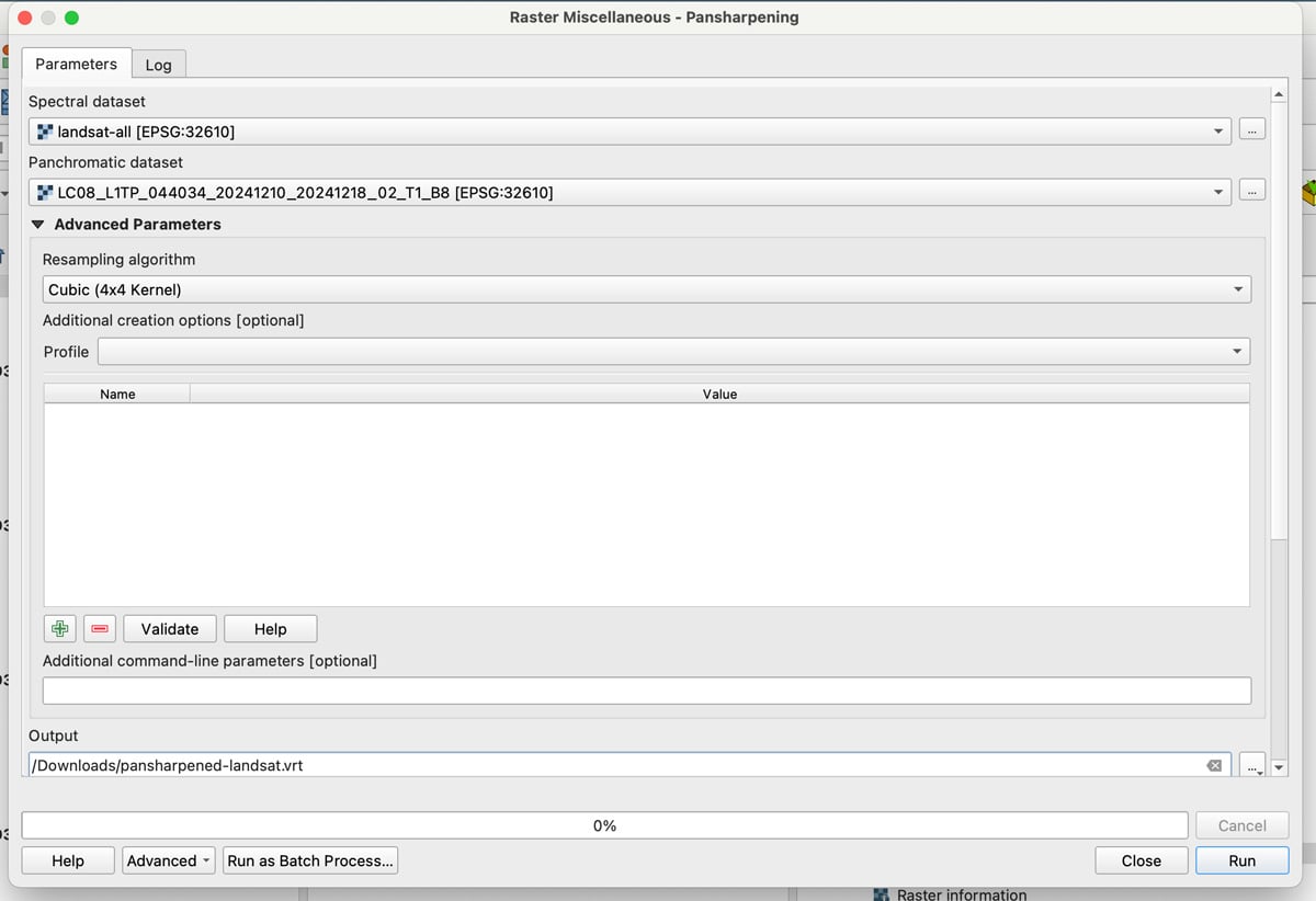
In the Pansharperning interface, select the merged multispectral image for the Spectral Dataset option. For the panchromatic, select the Landsat band 8 from the drop down.

Stay with the default Cubic resampling algorithm and then select a location on your computer to store the VRT file. Once all the parameters have been set, click the Run button.

The added 15 meter resolution VRT file with the sharper image will look identical to the original 30 meter resolution natural color image until you zoom in.