Air pollution is caused by both natural disasters and human activities. However, most of the pollutants in the atmosphere result from human activities, such as the emission of toxic gases by industries and harmful fumes from vehicles and trucks.
Although some substances are released by accident, others are deliberately emitted into the environment.
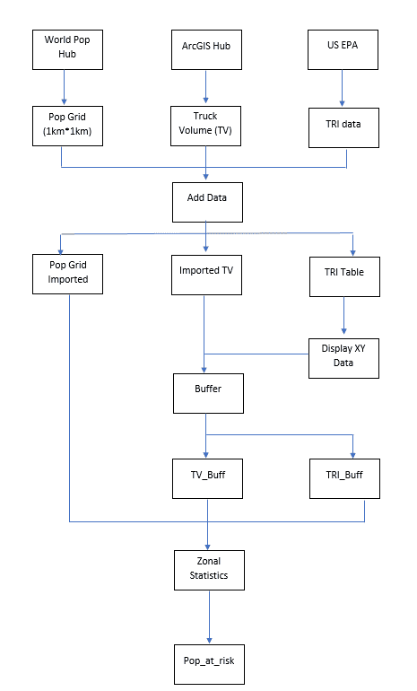
This tutorial shows how to use geospatial methodologies to estimate the number of people affected by air pollution using data from the Toxic Release Inventory (TRI), population grid data from Worldpop’s website, and truck volume information from the ArcGIS Hub.

Accessing and importing population data
To access population grid data for your desired area of interest, visit the worldPop’s website and follow the following steps:
- Select the data tab.
- Scroll through the data category page to select population count.
- Select the “unconstrained individual countries (1km resolution)” tab.
- Type and search desired country on the search bar to choose from the population inventory data. Since we are estimating population for Florida, type and search “United States 2020.”
- Click the option to access population grid data for United States 2020.

Next, import the population data into the ArcGIS Pro map canvas:
- Open and create a new project in ArcGIS Pro.
- From the Map tab of the menu bar, select the “Add Data” icon. Navigate to the Population grid data to be imported.
- Click OK.

Accessing and importing Toxic Release Inventory (TRI) data
To access the TRI data, visit United States Environmental Protection Agency (EPA)’s website: TRI Basic Data Files: Calendar Years 1987-Present.
- Choose a year and geographic area from the list of the drop-down menu. For this tutorial, we are selecting “FL” for Florida.

To import the Toxic Release Inventory (TRI) data into the ArcGIS Pro map canvas:
- Select the “Add Data” icon from the Map tab of the menu bar. Navigate to the TRI data to be imported.
- Click Ok.
The data is now imported as a table. To display the data based on its geographic coordinates:
- Right-click on the TRI layer from the Table of Contents panel.
- Select “Display X, Y Data.”
- Set X field to longitude and Y field to latitude.
- Click Ok.
Accessing and importing truck volume data
Access the Truck volume data from the ArcGIS data hub: Truck Volume TDA.
- Choose the Truck volume data in a shapefile format.
- Import the truck volume data into the ArcGIS Pro data view interface using the “Add data” tool from the menu bar icons.
- Click Ok.

Buffering TRI and truck volume data
A buffer distance of half a mile (802 meters) is created around the TRI data to estimate the number of people who are expected to be exposed to toxic gases.
To create a buffer around the TRI data;
- Type and search buffer from the search bar of the geoprocessing toolbar.
- Set input features to TRI data.
- Set Linear unit to meters.
- Set dissolve type to “dissolve all output features into a single output.”
- Click Run.

The formula below is also used to create a buffer around the truck volume data to estimate the number of people under pollution.
According to Karner et al. (2010)’s article,
Buffer distance for truck volume = 160 + ((TruckAADT-min)/max-min) * (570-160).
To create a buffer around the truck volume data in ArcGIS Pro;
- Right-click on the Truck volume layer and select “Attribute data” to open its attribute information.
- Create a new field with the field name “bufff_dist” and set data type to “float.”

- Sort the “TruckAADT” field as ascending and descending order to check the highest and lowest TruckAADT value.
- Right-click on the “bufff_dist” field and select “calculate field.”
- Type the formula as shown in figure 8 below.
- Click Ok.

- Type and search buffer from the search bar of the geoprocessing toolbar.
- Set input features to Truck volume data.
- Set Distance field to bufff_dist.
- Set dissolve type to “dissolve all output features into a single output.”
- Set “Output feature class” to desired output name and location.
- Click Run.

Zonal statistics to determine population at risk from TRI and truck volume data
To estimate the population at risk to toxic gases (TRI) in ArcGIS Pro;
- Type and search zonal statistics from the search bar of the geoprocessing toolbar.
- Set input feature data to TRI_buff data.
- Set Zone field to OBJECTID.
- Set “Output Raster” to desired output name and location.
- Set Statistics type to “Sum.”
- Click “Run.”

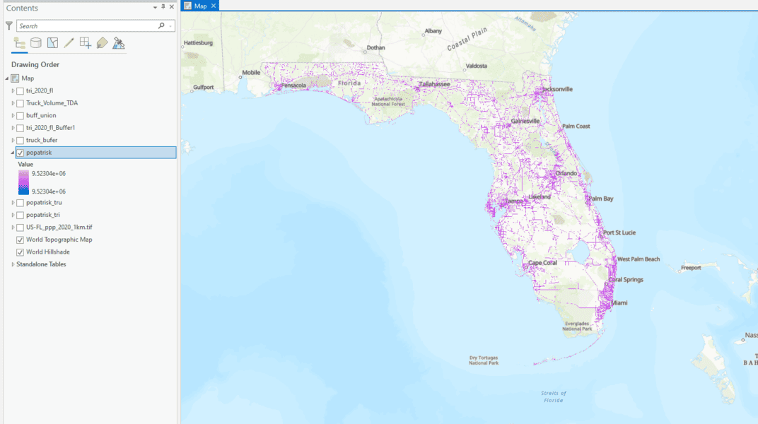
Repeat the steps to calculate zonal statistics for truck volume to estimate the population exposed to pollution from trucks.
To estimate the population exposed to pollution from trucks and toxic gases;
- Type and search “union” from the search bar of the geoprocessing toolbar.
- Set input features to TRI_buff and truck _buff data.
- Set “Output Raster” to desired output name and location.
- Click “Run.”

- Type and search zonal statistics from the search bar of the geoprocessing toolbar.
- Set input feature data to TRI_buff data.
- Set Zone field to OBJECTID.
- Set “Output Raster” to desired output name and location.
- Set Statistics type to “Sum.”
- Click “Run.”

References
Karner, A. A., Eisinger, D. S., & Niemeier, D. A. (2010). Near-Roadway Air Quality: Synthesizing the Findings from Real-World Data. Environmental Science & Technology, 44(14), 5334–5344. https://doi.org/10.1021/es100008x
