
Groundwater potential zones are areas with subsurface water content. This study is aimed at exploring the efficacy of geoinformation tools and open-source data for assessing groundwater potential in deserts.
The study area is located in the dry western parts of Rajasthan, covering 12000 square km in the Jaisalmer district and the data used are:
- Geocoded Survey of India (SOI) Topographical Maps
- RESOURCESAT-1-LISS-III from Bhuvan
- ALOS-1 PALSAR data from NASA Earthdata
- ASTER GLOBAL DEM from USGS Earth Explorer data
This study attempts to apply an integrated approach of remote sensing and GIS for generating five thematic data layers for the delineation of potential groundwater zones.
The five thematic layers: Buffers (potential water sources such as natural streams, lakes/ponds, canals and lineaments), land use and land cover (LULC), NDVI, Slope and Depression are taken into account for the determination of groundwater potential.

Steps
In the first step, SOI Topographical sheets of 1:50,000 were converted to the digital format by scanning in TIFF format and geo-referenced into Universal Transverse Mercator (UTM), spheroid and datum WGS-1984 42N. All well locations were digitized using ArcMap 10.1.
The second step utilized LISS III to generate LULC using a hybrid classification technique using ERDAS Imagine 2011. The study area was classified into sand which covered significant portions, waterbody, canals, cultivated land, vegetation, settlement, hills and salt and gravel wastes.
The third step involved the generation of NDVI in ERDAS. It is used to determine the density of a green patch of land.
The fourth step involved creating Slope and Depression maps using ASTER GLOBAL DEM using 3D Analyst tools in ArcMap 10.1 and Model Maker in ERDAS 2011, respectively.
The fifth step utilized ALOS-1 PALSAR level 1.5 dual-polarization (HH and HV) data which was processed in PolSARPro software using different edge detection filtering methods like Sobel, Laplace, differential, gradient, etc. to enhance ALOS-1 PALSAR polarimetric data for lineament detection. Finally, lineaments were marked using the visual interpretation of the LISS-III image and HH and HV polarization images utilizing the optical image and the mentioned enhancement technique.
The sixth step involved preparing buffer layers for natural streams, canals, bunds, lakes/ponds and lineaments. Buffers were created using proximity analysis tools in ArcMap 10.1 after digitizing all the mentioned layers. For Lakes/ponds 1km, natural streams 1 km, canals 0.5 km, bunds 1 km and lineaments, 0.5 km buffer was given. All maps were converted to raster format for weighted overlay analysis.
Overlay Analysis
Overlay analysis for groundwater potential map was done in Model Maker of ERDAS 2011, using weighted linear combination technique. Weighted overlay only accepts rasters as input. The evaluation scale chosen for each class in a thematic layer was 10 and for all thematic layers was 5.
Each input raster was weighted or assigned a value of influence out of 5 based on its importance in controlling the groundwater potentiality in this region. Along with the raster themes, individual classes within a raster were also given ratings based on their influence out of 10 in groundwater potentiality in the given study area.
A relative score of each thematic unit in a theme was calculated by multiplying the weight of the theme with the rate of the respective thematic unit. Finally, generated groundwater potential map was categorized into low (0-30 total weight), medium (30-60 total weight), high (60-90 total weight) and very high (>90 total weight).
The weight/ratings of each layer/class are given in table 1. The groundwater potential map prepared in this process were validated by overlaying it with the well locations as marked from the SOI Maps.
| Thematic Layers | Weight |
| Water sources and lineaments | 5 |
| LULC | 4 |
| NDVI | 3 |
| Slope | 2 |
| Depression | 1 |
Ratings for each class in the thematic layers are shown in tables 2 to 6:
| Lakes/Ponds etc. | 10 |
| Lineaments | 8 |
| Canals | 8 |
| Bunds | 7 |
| Waterbody | 10 |
| Canal | 8 |
| Vegetation | 7 |
| Settlement | 6 |
| Agriculture | 5 |
| Salt and Gravel Wastes | 3 |
| Hills | 1 |
| Sand | 1 |
| > 0.1 to < 0.6 | 7 |
| >= 0.6 to 1 | 10 |
| -1 to 0.1 | 1 |
| 0 -5 | 10 |
| 5 – 15 | 8 |
| 15 – 25 | 6 |
| 25 – 35 | 3 |
| >35 | 1 |
| >= 5m | 10 |
| >0 to 5m | 5 |
| =0 | 1 |
Results and Discussion:
Drainage Buffer:
“It is well known that the denser the drainage network, the lesser is the recharge rate and vice versa” (Edet et al. 1998). Drainage is divided into water bodies like lakes and ponds, natural streams, canals, and bunds in the study area.
Weights are given to each buffer zone as given in table 2, shown in figures 2a and 2b.

Lineament Buffer:
“Presence of lineaments can act as a conduit for groundwater movement, resulting in increased porosity and, therefore, serve as a prospective groundwater zone” (Obi Reddy et al., 2000). Similarly, intersections of lineaments are also probably sites of suitable groundwater prospective zones. Most of the lineaments lie on the North-West portion and are North-East aligned in the study area, as shown in figures 3a and 3b.

Land-use and Land-cover:
The effect of LULC is manifested either by reducing runoff or by trapping water by plants. LULC may also affect groundwater negatively by evapotranspiration, assuming interception to be constant. The presence of vegetation suggests the presence of groundwater for plants to survive.
The same goes for agriculture which requires a sufficient amount of groundwater. People tend to settle in proximity to water, so a high weightage is given to the settlement class. This is shown in figure 4a.
NDVI:
It is used to determine the density of a green patch of land. Thus, a higher NDVI value shows more possibility of the presence of groundwater in the region as shown in figure 4b.

Slope:
Concerning groundwater, where the slope is high, there will be high runoff and low infiltration. Figure 5a shows the slope map of the study area.
Depression:
ASTER GDEM is used to generate depression zones using a simple subtraction technique of filled DEM and raw DEM. The output shows various depression zones all over the study area, such as in interdunal spaces and salt waste/gravel waste zones. This is shown in figure 5b.

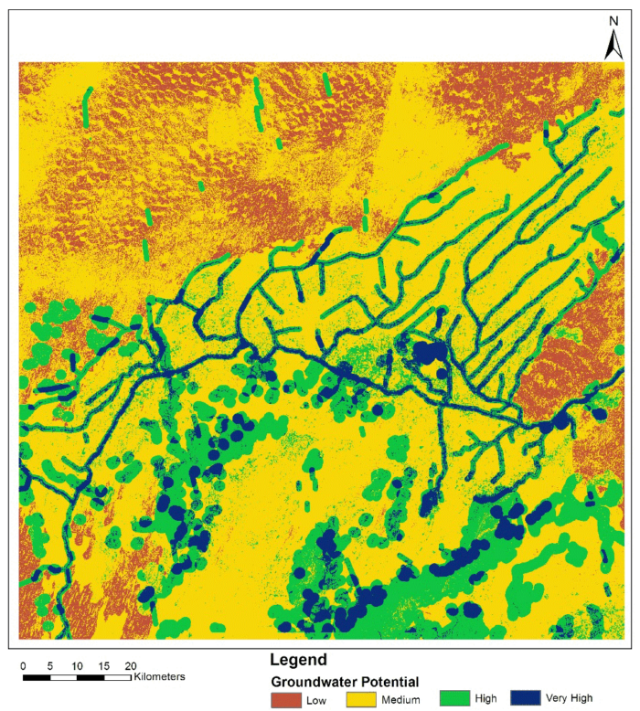
Groundwater Potential Map:
After integrating all maps in weighted overlay analysis, the final groundwater potential map is prepared. Based on the total weight, the groundwater potential of the study area is divided into low, medium, high and very high potential.
Most groundwater potential zones are found to be concentrated near the lineament and water sources of the study area. Also, the higher potential is observed near vegetation cover and cultivated lands and near settlements. The least potential is observed in the sand cover and on the hills. This is shown in figure 6.

The generated groundwater potential map is validated through the location of wells extracted from geocoded toposheets and the well location data obtained from CGWB (Central Ground Water Board). The well locations are depicted in figure 7.
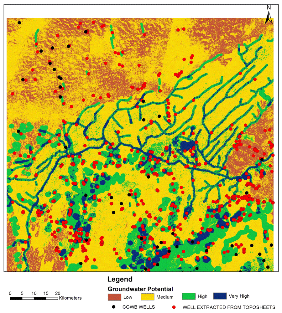
The number of well locations in different groundwater potential categories has been presented in table 7.

The table indicates that almost 50% of wells are in high to very high groundwater potential zone, and about 40% of the rest of the wells are in medium groundwater potential zone.
This implies that the methodology followed in the present study for groundwater potential has good predictability and potential for future work in deserts.
References
Reddy, G. O., Mouli, K. C., Srivastav, S. K., Srinivas, C. V., & Maji, A. K. (2000). Evaluation of groundwater potential zones using remote sensing data-A case study of Gaimukh watershed, Bhandara District, Maharashtra. Journal of the Indian Society of Remote Sensing, 28(1), 19-32. https://doi.org/10.1007/BF02991858
Edet, A. E., Okereke, C. S., Teme, S. C., & Esu, E. O. (1998). Application of remote-sensing data to groundwater exploration: a case study of the Cross River State, southeastern Nigeria. Hydrogeology Journal, 6(3), 394-404. https://doi.org/10.1007/s100400050162
About the Author
Anindita Ghosh is a Geographer and Planner with a keen interest in spatial analysis. Her expertise lies primarily in research, data analysis, and application of GIS in urban studies. Her areas of interest include policy research, climate change, urban flood, resilient cities and regional planning.
Anindita has completed her M.Phil. in Urban and Regional Planning from CEPT University, Ahmedabad and is currently a PhD student at the Symbiosis Institute of Geoinformatics, Pune.
Anindita can be reached via email.