Welcome to another tutorial about tackling common GIS problems! In the previous one, I showed you a method for automatically reclassifying a continuous raster to discrete values, using Arcmap’s model builder. Today, we will work on something that is more oriented towards Urban Planning applications, and that is calculating Land Use Mix.

Land Use Mix indicates the level of diversity of land use types within an area and it is an important aspect of Urban Planning and Spatial Planning. For example, the policy of mixed land use is considered an important component for promoting walkability in an urban area (Mavoa et. al., 2018) and it is considered to be energy-efficient (Zhang & Zhao, 2017). 

However, it was observed that no tool has been developed so far in the field of land use mix calculations, neither as standalone, nor as part of existing GIS software. For this purpose, I developed a Python script in the form of a Jupyter notebook that can make the appropriate calculations. You can check it out on my Github’s Land Analyzer page. On this page you can also find one of the datasets we are going use in this example. 

In the documentation page, I explain how the script works and present some results, but I do not get into much detail regarding the GIS algorithm required to make the calculations. This article will be devoted to that, and we will calculate Land Use Mix indices with step-by-step instructions using QGIS. The proceedure is perfectly reproducible in other GIS software too.

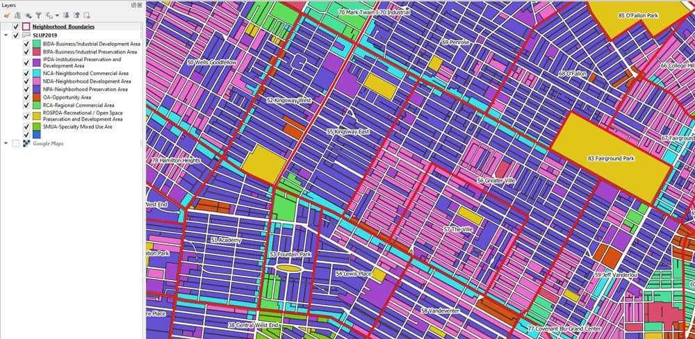
Let’s start with an overview of our datasets. I have downloaded a Land Use dataset for the city of Saint Louis, Missouri. For the same city, we have a shapefile of the neighborhoods of the center. Our goal is to calculate the land use mix for each of those neighborhoods. 

Entropy Index for Land Use Mix

Before we begin, we need an index that will quantify this mix. Entropy index is a commontly used metric to do this (Song et. al., 2013):

where P^j, is the percentage of each land use type j in the area and k is the total number of land use types. 

The percentage P^j  is calculated in terms of area. As an example, consider an area with a total of 3 land use types:

• Residential, covering 50% of the area
• Industrial, covering 20% of the area
• Commercial, covering 30% of the area, then:

k=3 and P¹ = 0.5, P² = 0.2 and P³ = 0.3

Use the Intersect Tool to Associate Land Use with Neighborhoods

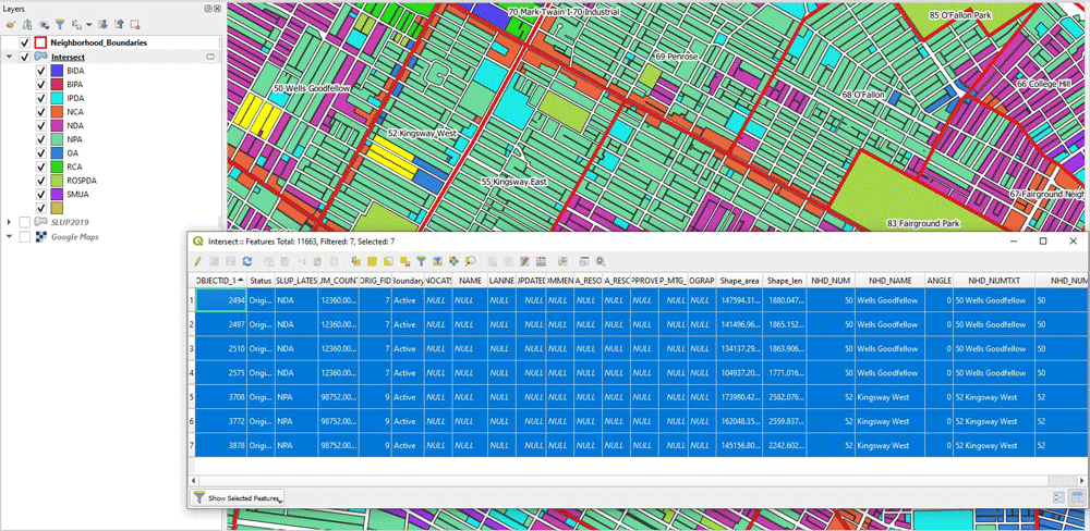
As you understand, the crucial part is to calculate the P^Js. In order to do that, the features of the land use dataset must be attributed with the neighborhood feature they belong to. To do that, we use the Intersect tool. In the next two figures, you can see the parameters we set to run the tool (note: I will always use temporary outputs except for the final one, in order to save time) and the outcome itself. In the outcome, notice the 7 selected polygons. The new columns in their attribute table indicate which neighborhood they belong to. 

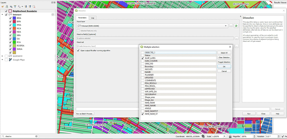
Next, for each land use type we need to calculate the proportion of its area to the total area of the neighborhood. To do that, it’s useful to have all the polygons of each type as one multi-polygon. To do that, we use the Dissolve tool in QGIS.

We dissolve based on two columns: the land use type (SLUP_LATES) and the neighborhood identifier column (NHD_NUM_ST). By doing so, we merge together all the polygons of the same type of the same neighborhood. In the outcome, notice how the selected polygon refers to all the polygons of type “NPA”, within the boundaries of Neighborhood 50.

(Note: if you get an error at this point, using this particular dataset, don’t worry about it. Some polygons are invalid and though it does affect the numerical outcome, it doesn’t prevent us from understanding the steps of the algorithm)

Calculate the Area of Each Land Use Type Multi Polygon

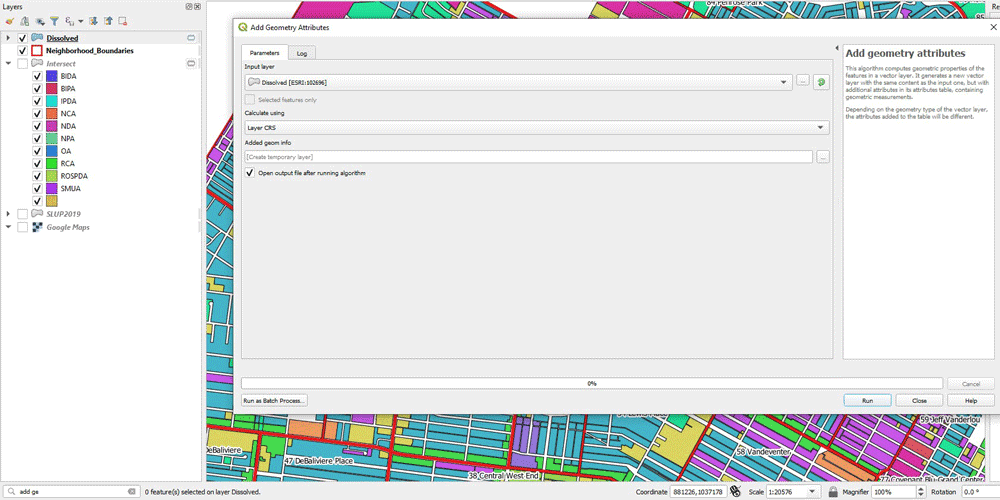
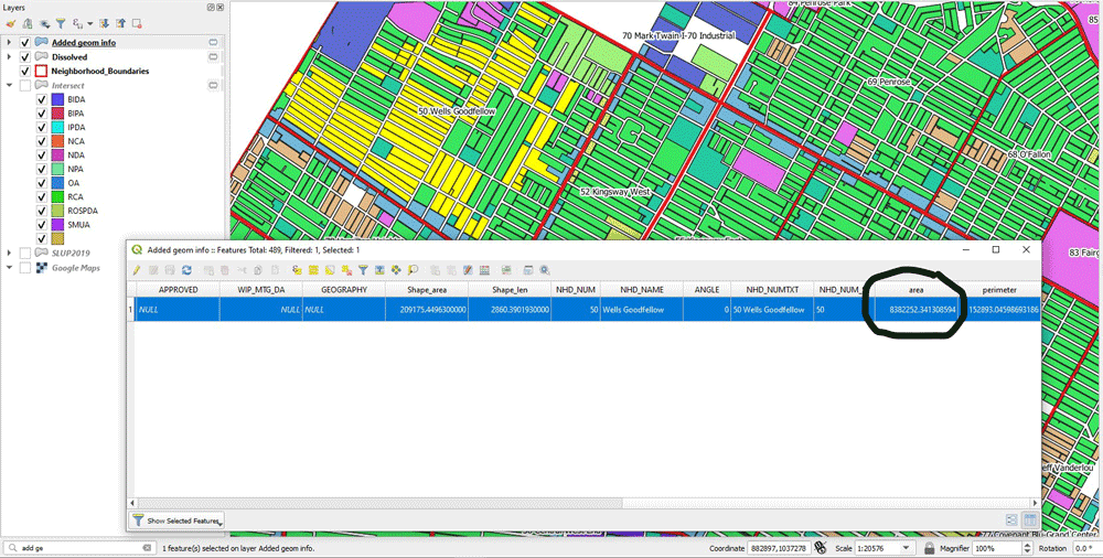
Now, the next step is to calculate the areas. We need to calculate the area of each land use type multi polygon, as well as the area of the neighborhood polygon in which it belongs to. For this, we use “Add geometry attributes”. We do that for both of the outcome of Dissolve, as well as the Neighborhoods layer. 

Joining the Layers

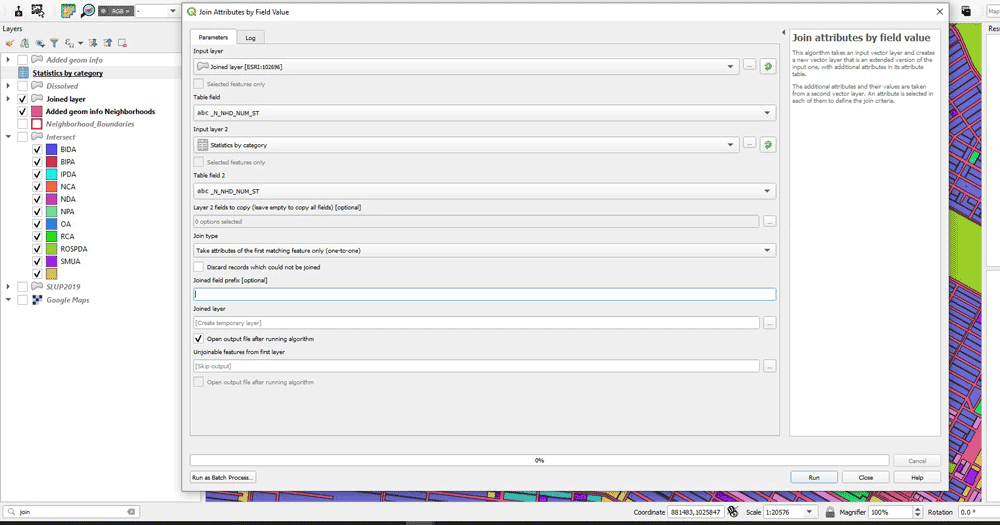
Since we need to calculate the ratio P^J, we need to bring together these two pieces of area information. We have calculated the areas for both layers. In the next figure, it’s the layers “Added geom info” and “Added geom infor Neighborhoods”. We need to join these two together, and we do it with “Join Attributes by Field Value”. We need to set the input layers and the field upon which they will be joined. Also notice I use a prefix for the joined fields (“_N_”). In the output, we have the land use layer joined with the neighborhoods layer and there is area information for both the polygon (“area” column) and the neighborhood polygon it belongs to (“_N_area”).

Statistics by Categories Tool

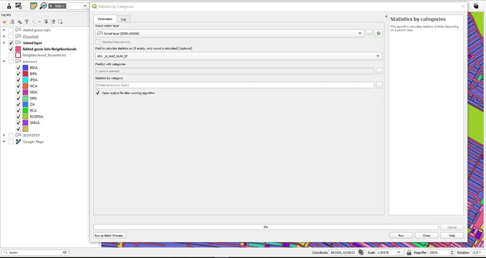
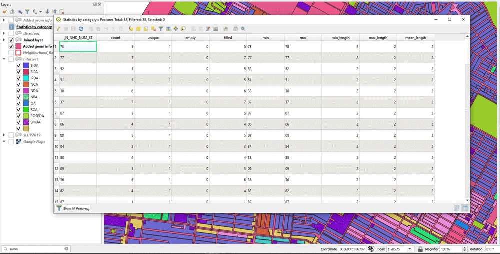
However, except for the areas, we need to calculate the total number of land use types that are contained in each neighborhood polygon. We  can use Statistics by Categories tool for the Joined layer. We just select the “N_NHD_NUM_ST” column to calculate statistics on and we use the same as the Field with the categories. This will produce an output were for each neighborhood polygon, the total number of included land use types have been calculated. This is the layer “Statistics by category”.

Joining All the Information Into One Layer

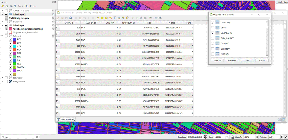
Next, we need to join this new layer with the previous layer too. This is done to have all the information needed in one layer: Total area of  each land use type, area of the neighborhood they  belongs too, and total number of land use types within that neighborhood. As an additional step, I use Organize Columns in the attribute table to keep only the desired columns. Those are the columns “area”, “_N_area” and “count”.

Calculating the Entropy Index

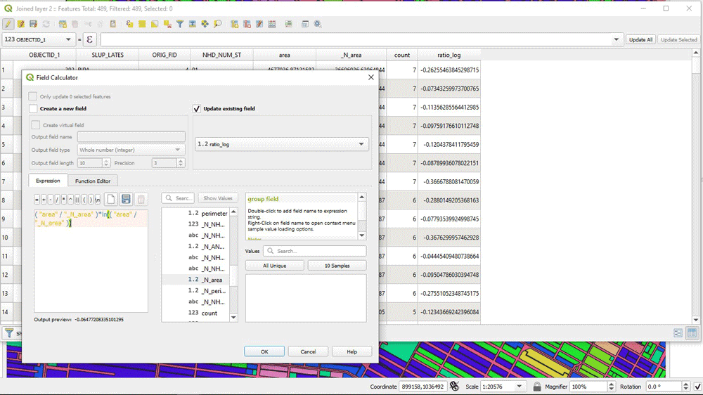
Next, by creating a new column (“ratio_log”), we can do the main calculation for the Entropy index. That is the product:

We use the following expression to do that:

( “area” / “_N_area” )*ln(( “area” / “_N_area” ))

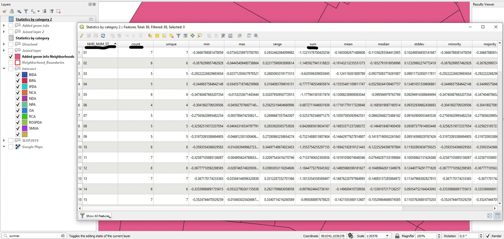
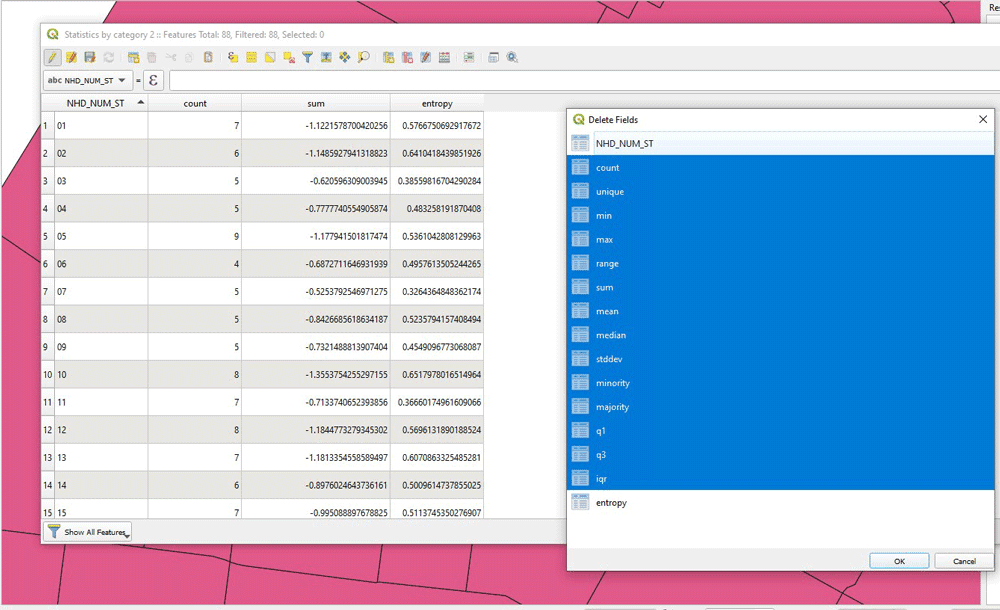
The next part is to sum the “ratio_log” column based on the land use type. So, we use again “Statistics by categories”. We use the “ratio_log” as the field to calculate statistics on and we select the “NHD_NUM_ST” as the Field with categories.  From the output, we care about the columns “NHD_NUM_ST” (each neighborhood), “count” (total number of land use types) and “sum” (the sum of the product calculated above).

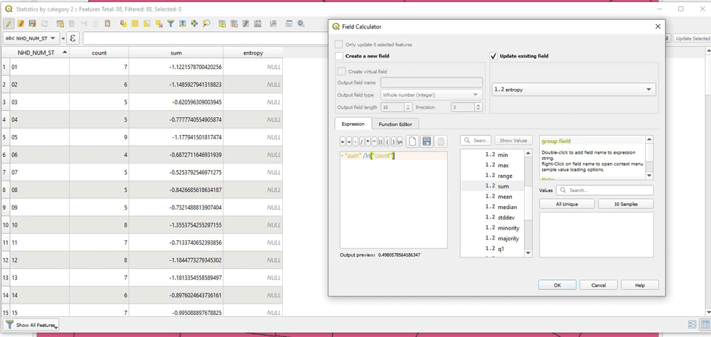
As a final step for calculating the entropy, first we keep only those fields, and then we make a new column to calculate the entropy. We use the field calculator to make the final calculation as follows:

-“sum”/ln(“count”)

Join the Entropy Table with the Neighborhoods Layer

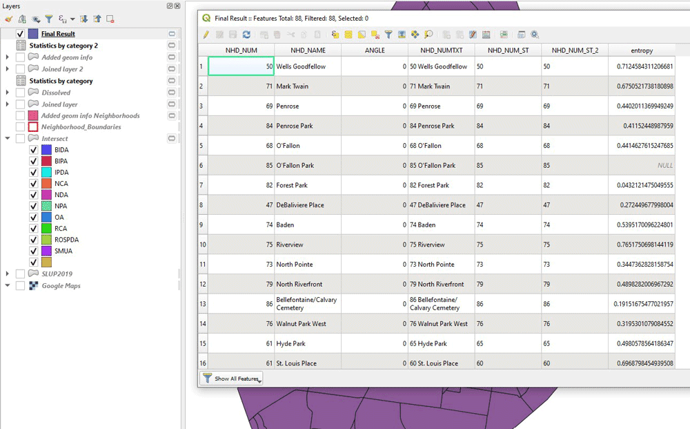
Now, we have the entropy calculated for each neighborhood polygon, but that’s in a tabular layer, derived from Statistics by Categories. We join that to the original Neighborhoods layer and our work is complete!

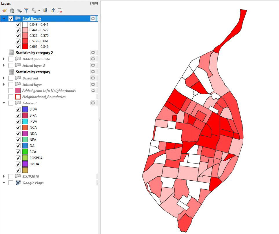
Mapping Land Use Entropy Index in a Neighborhood

We can take a look at the result as a final map, to see which neighborhoods have the highest entropy. 

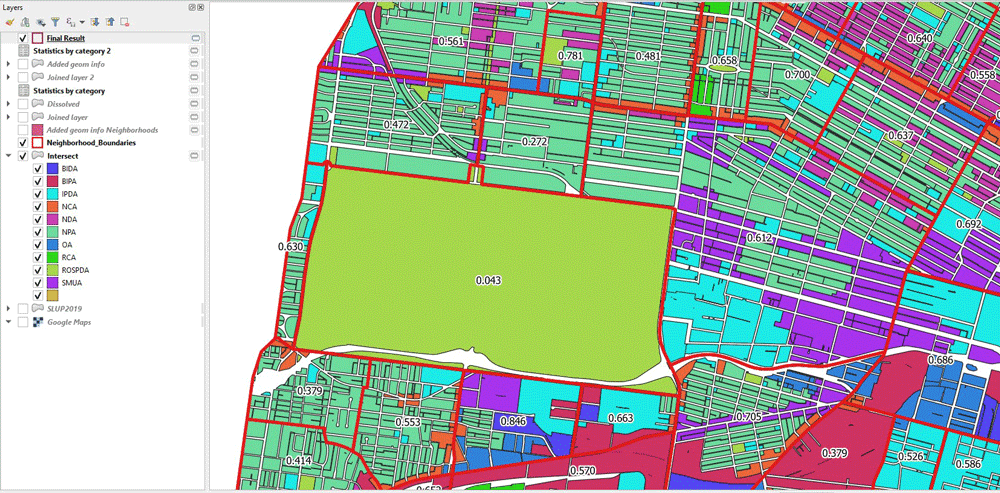
As a reality check, we can zoom into an area in more detail and use the entropy as labels for each neighborhood polygon. We can see indeed that a neighborhood containing only one land use type has very low entropy (essentially 0), while the surrounding ones have higher entropy. 

That’s the whole process for calculating entropy index for an area using qgis. It might seem a bit complicated with all the layers and screenshots, but it really is a simple series of steps, once you understand what calculations you need to make. However, if you lost me on any part of the process, feel free to contact me. If you don’t have any questions but just want to provide some feedback, this is also welcome.

About the Author

Alexandros Voukenas received his diploma (MSc equivalent) in Surveying Engineering from Aristotle University of Thessaloniki in 2017 and has been working as a GIS & Remote Sensing Engineer in the private sector ever since. His main areas of occupation have been the production of reference mapping using Geographic Information Systems and satellite imagery, and to perform feasibility research studies on remote sensing projects. Voukenas is passionate about solving of real life problems and he has won a prize in four innovation hackathons, including the Fabspace 2.0 Greece (1st place), the NASA Space Apps Challenge Thessaloniki (2nd place) and the Crowdhackathon smarticity (4th place). He is also an active researcher on the topics of urban data analysis and remote sensing. His other research interests are spatial analysis & statistics, GIS, geospatial technologies, photogrammetry and computer vision. Alexandros Voukenas can be contacted via email.

More from Alexandros Voukenas:

• Automatic Raster Reclassification with ArcMap Model Builder Based on Raster Statistics

Literature

Mavoa, S. et al., 2018. Identifying appropriate land-use mix measures for use in a national walkability index. The Journal of Transport and Land Use, 11(1), pp. 681-700.

Song, Y., Martin, L. & Rodriguez, D., 2013. Comparing measures of urban land use mix. Computers, Environment and Urban Systems, Volume 42, pp. 1-13.

Zhang, M. & Zhao, P., 2017. The impact of land-use mix on residents’ travel energy consumption: New evidence from Beijing. Transportation Research Part D, Volume 57, pp. 224-236.

Related

• How to Measure “Land Use Mix” using Entropy in Maptitude
• 2020 Global Land Use Data
• How to Use ArcGIS Pro to Map Urban Heat Islands
• USGS Releases Two Decades of Land Cover Change for the Contiguous United States