
One of the emerging technologies that steers that frontier of urban development and land use planning is geospatial tools and methodologies.
Remote sensing provides a proactive way of addressing issues by implementing its data collection, processing, and map presentation techniques in solving a wide range of problems that affects the environment, health, safety, transportation, land use demarcation, among several others. Satellite imagery has been used substantially in the land use management and planning arena for the management and monitoring of land systems.
This tutorial contributes to the several land use assessment and management techniques in the geospatial industry by presenting a step-by-step approach of applying Remote Sensing and GIS techniques to perform supervised classification on Landsat 8 imagery. Even though several classification algorithms have evolved over the years, this tutorial utilizes the Maximum Likelihood algorithm.
Figure 1 shows a summary of the methodological flow employed in performing supervised classification in ArcGIS Pro.

Landsat Imagery and Creating Composite Bands
For the purposes of this tutorial, Landsat 8 imagery is accessed from the USGS Earth Explorer’s website, after a free sign-up process.
Cloud cover for the Landsat 8 imagery should be set to “less than 10 percent.” To correct for atmospheric errors, the following video is helpful: Satellite Imagery Cloud Removal and Correction In ArcGIS Pro.
The following band combinations may be used for band compositing processes; natural color (bands 4,3,2), false color (bands 7,6,4), color infrared (bands 5,4,3), among many others. These band combinations make it easier to detect specific land use classes during sample training for classification. For this tutorial, (bands 5,4,3) are used.
To perform band compositing in ArcGIS Pro, the following steps are adhered to:
- Open ArcGIS Pro and create a new project.
- From the Map tab, select “Add data,” and navigate to the location of the Landsat 8 imagery.
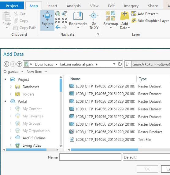
- Select Bands 5,4,3 and click “Ok.”
- From the search bar of the geo-processing toolbox, type and search “Composite bands.”
- Set “Input Raster” to bands 5,4,3.
- Set “Output Raster” to the desired output name and location.
- Click “Run.”

Clipping, Training Sample Manager, and Classify
To streamline the Landsat imagery to a desired area of interest, the following steps are followed;
- Type and search “Extract by Mask” from the search bar of the geo-processing toolbox.
- Set “Input Raster” to the stacked image (results obtained from the composite band process).
- Set “feature mask” to the desired area of interest.
- Set “Output Raster” to the desired output name and location.
- Click “Run.”

To train sample data for classification in ArcGIS Pro, the following steps are followed;
- From the drop-down menu of “Classification Tools” on the Imagery tab, select “Training Samples Manager.”
- From the “new schema” tab, select “Edit Properties.”
- Set “name” to desired schema output name, and click “Save.”

New classes can be added to the schema, and training data can be selected by;
- Select “Add New Class” as shown in figure 5 above.
- Set “Class Name” and “Value” to the intended class to be trained.
- Click “Ok.”
For this tutorial, the following classes are used; dense forest, open forest, water, and built-up areas. To select training samples for water;
- Click water from the schema panel and select a drawing tool.
- Hover the mouse pointer over the stacked imagery while sketching over water bodies in the area of study.
- Repeat steps for other land use classes; open forest, dense forest and built-up areas.
- To save the training samples, click “save as” as shown in figure 6.

To classify the Landsat imagery using the collected and saved training sample data, the following steps are used;
- From the drop-down menu of “Classification Tools” on the Imagery tab, select “Classify.”
- From the “Classify” interface, set classifier to maximum likelihood.
- Set “training sample” to results of the “training sample manager.”
- Click “Run.”

The end result is this classified layer that you can then stylize:

Accuracy Assessment of Classified Image in ArcGIS Pro
To validate the classification results, the following steps are followed;
- Type and search “Create Accuracy Assessment Points” from the search bar of the geo-processing toolbox.
- Set “Input Raster” to the classified image.
- Set “Output Accuracy Assessment Points” to the desired name and location of the automatically generated accuracy assessment points.
- Set “Number of Points” to 500 and Sampling strategy to “Stratified Random.”
- Click “Run.”

- Open the attribute table of the generated accuracy assessment points.
The default ground truth values for the data points as shown in the attribute table are -1.
- Click on the “Edit” tab from the menu bar.
- Set the ground truth values for each of the accuracy assessment points (500) by matching the points to the land use class of the base map.
- Turn the column which represents the values of the various land use classes of the “Classified image” upon which these accuracy assessment points were generated off while undertaking step 8.
- Save changes.

To generate a confusion matrix from the accuracy assessment points, the following steps are followed;
- Type and search “Compute Confusion Matrix” from the search bar of the geo-processing toolbox.
- Set “input accuracy assessment points” to the generated accuracy assessment points and set “output confusion matrix” to the desired name and location of the matrix.
- Click “Run.”
Table 1: Confusion matrix of classification
| ClassValue | Water | Open forest | Dense forest | Built up areas | Total | U_Accuracy | Kappa |
| Water | 10 | 0 | 0 | 0 | 10 | 1 | 0 |
| Open forest | 5 | 194 | 4 | 0 | 203 | 0.95566502 | 0 |
| Dense forest | 1 | 7 | 237 | 1 | 246 | 0.96341463 | 0 |
| Built up areas | 0 | 2 | 1 | 46 | 49 | 0.93877551 | 0 |
| Total | 16 | 203 | 242 | 47 | 508 | 0 | 0 |
| P_Accuracy | 0.625 | 0.9556 | 0.97933 | 0.97872 | 0 | 0.958661417 | 0 |
| Kappa | 0 | 0 | 0 | 0 | 0 | 0 | 0.93111 |
More ArcGIS Pro Tutorials
- How to Use ArcGIS Pro to Estimate Soil Erosion from a Catchment Basin
- How to Use ArcGIS Pro for Fire Risk Mapping
- How to Use ArcGIS Pro for Automatic Shoreline Delineation from Landsat Imagery
- How to Use ArcGIS Pro to Map Urban Heat Islands
- How to Use ArcGIS Pro to Calculate Land Surface Temperature (LST) from Landsat Imagery