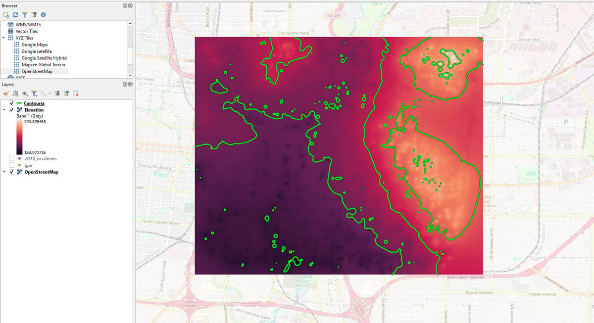
As a fundamental geospatial method, interpolation is one of the most crucial tools in QGIS for making complex surface layers with contours. This method uses the power of spatial data to create continuous representations that clearly show changes in elevation, temperature gradients, rainfall patterns, and other things that happen in different places.
What is interpolation in GIS?
For the most part, interpolation in GIS is a way to find unknown values across an area of geography by using known values from a GIS dataset. This method turns discrete point datasets—like elevation points from topographic surveys, weather sites, or satellite observations—into complete surface models. When these models are overlaid with contour lines, they tell a visual story that shows how terrains, climate changes, or any other topographic feature relates.
Performing interpolation in QGIS
In QGIS, the interpolation process is composed of several carefully planned steps. This GIS tutorial will guide you through finding elevation data, loading point datasets into QGIS, selecting an applicable interpolation method, creating a surface layer from those elevation points, and checking the output layer for accuracy and completeness.
Creating topographic contours in QGIS
After the interpolation process completes and an output raster surface shows the continuous spatial characteristic, the next important step is to create contours. When you look at interpolated surfaces as contours, you can easily understand how elevation or attribute changes happen across regions. These contour lines are automatically made by QGIS, and users can choose the contour intervals that best show the details of the spatial phenomenon they are looking at.
When you use interpolation and contour generation together in QGIS, you can make layers that are both visually appealing and full of useful information. These layers, full of detailed contours on top of finely interpolated surfaces, help GIS professionals, scientists, and decision-makers figure out complex spatial patterns, do more accurate analyses, and learn more about the many factors that affect our surroundings.
Tutorial Overview for creating a surface layer and contours in QGIS
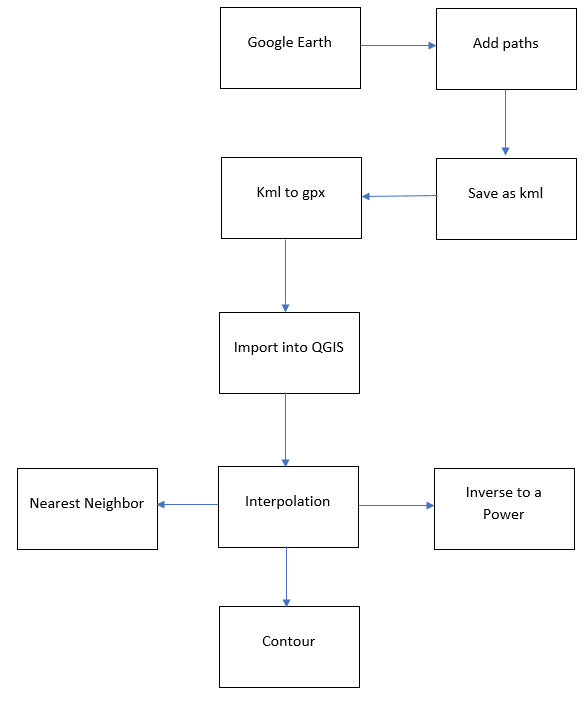
For this tutorial, “add paths” in Google Earth Pro was used to digitize lines over our area of interest (San Antonio, TX, USA). The resulting file was saved in a .kml format. GPS Visualizer’s portal was used to convert these lines (.kml) into a .gpx file. The file was imported as points into QGIS canvas. Surface raster files (Grid Nearest Neighbor and Inverse to a Power) were created over the .gpx points using the elevation field with contours.
Using elevation data from Google Earth Pro
For this tutorial, we will be using Google Earth Pro’s offline installer or online installer: Earth Versions – Google Earth. You have installed Google Earth Pro on your computer:
- Launch Google Earth Pro.
- From the pool of icons, select “add paths” and digitize randomly over your area of interest.
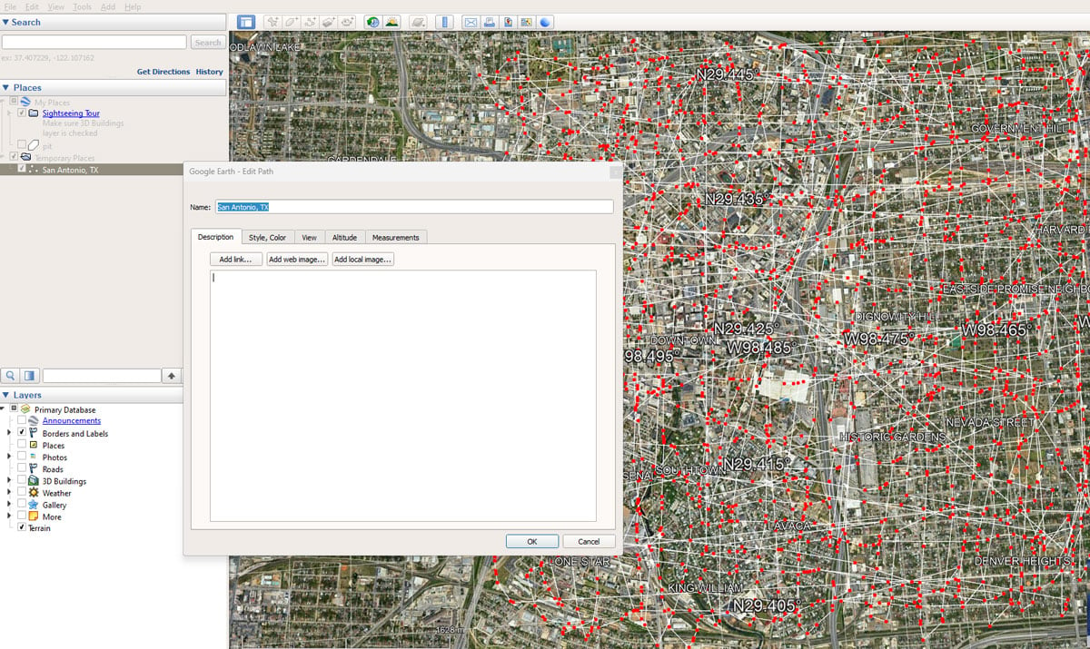
- After digitizing over the area, set Name to San Antonio, TX and click Ok.
- From places window, right-click on digitized file and select “Save place as”.
- Toggle to your desired output location and set output.
- Click Ok to save the digitized KML file.
Use GPS Visualizer to extract elevation data
- In a web browser, open the GPS Visualizer website.
- Select “choose file” to upload the digitized KML file.
- Click “Convert and add elevation.”

- Click the download button to retrieve the converted .gpx file.
use QGIS to add the geospatial data
Start a QGIS project. Next, add Open Street map as a base layer by:
- Selecting the Manage and install plugins from the Plugins tab.
- Type and search Quick Map services from the search bar.
- Click install.
- From the web tab, select QuickMap services.
- Select OSM to import the OSM map onto the QGIS map canvas.
To import the elevation data (.gpx) file into the map canvas:
- Set Vector dataset to the .gpx file.
- Select Add.
- A window appears requesting your desired vector file format.
- Select Points and select Add layers.

Create a surface layer in QGIS from elevation data
QGIS has many interpolation methods, and each works with a different set of data and spatial setups. Different techniques, such as Inverse Distance Weighting (IDW), Kriging, TIN interpolation, and Spline interpolation, each have their benefits. For example, some can handle points not spread out evenly, others can handle spatial correlations, and others can make smooth, continuous surfaces.
Here are two of the ways you can use the tools in QGIS to create a surface layer from elevation data.
Approach 1: Grid (Inverse to a Power)
The “Grid (Inverse to a Power)” tool in QGIS is a type of Inverse Distance Weighted (IDW) interpolation. This tool estimates unknown values (like elevation) at specific locations based on known values from surrounding points. This estimation takes into account the distances between known and unknown points, with closer points usually having more influence than those farther away. The “inverse” in the name refers to this relationship: as distance increases, the influence or weight of a point decreases.
This method is particularly useful when you have a scattered set of points with known values (like elevation data from a survey) and you want to create a continuous surface that estimates values between these points.
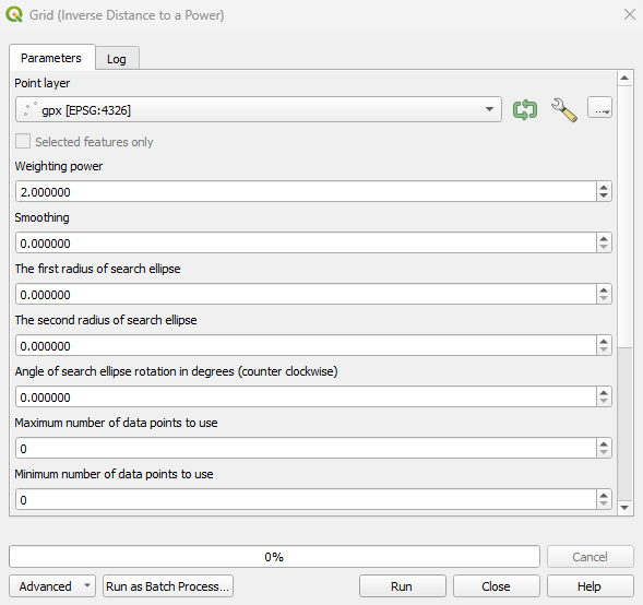
To create a surface layer (Grid (Inverse to a Power)) the .gpx points using the elevation field:
- Select Raster from the menu tools.
- Select Analysis.
- Select “Inverse Distance to a Power.”
- Set the point layer to gpx points.
- Click the Advanced Parameters from the Grid window.
- Set z field to “ele.”
- Set the output file to your desired output name and location.
- Click Run.
Approach 2: Grid (Nearest Neighbor)
Alternatively, a surface raster can be created using the Grid (Nearest Neighbor) algorithm or Thiessen polygon which is part of the GDAL grid utility. The “Grid (Nearest Neighbor)” tool in QGIS applies the nearest neighbor method to interpolate values for each cell of the output raster. For each cell in the output grid, the tool assigns the value of the closest input data point. This method is particularly useful when you have a set of discrete data points and you want to create a continuous surface, such as an elevation model.
To create a surface layer using the “Grid (Nearest Neighbor)” tool:
- Select Raster from the menu tools.
- Select Analysis.
- Select “Grid (Nearest neighbor).”
- Set the point layer to gpx points.
- Click the Advanced Parameters from the Grid window.
- Set z field to “ele.”
- Set the output file to your desired output name and location.
- Click Run.

Applying symbology to the GPS points layer to validate the results of the surface Layer
To visualize and validate the results of our output surface layer, we will classify our gpx points. This allows us to scan the resulting surface layer to make sure the assigned elevation values of the raster data align with the elevation values of the input point data:
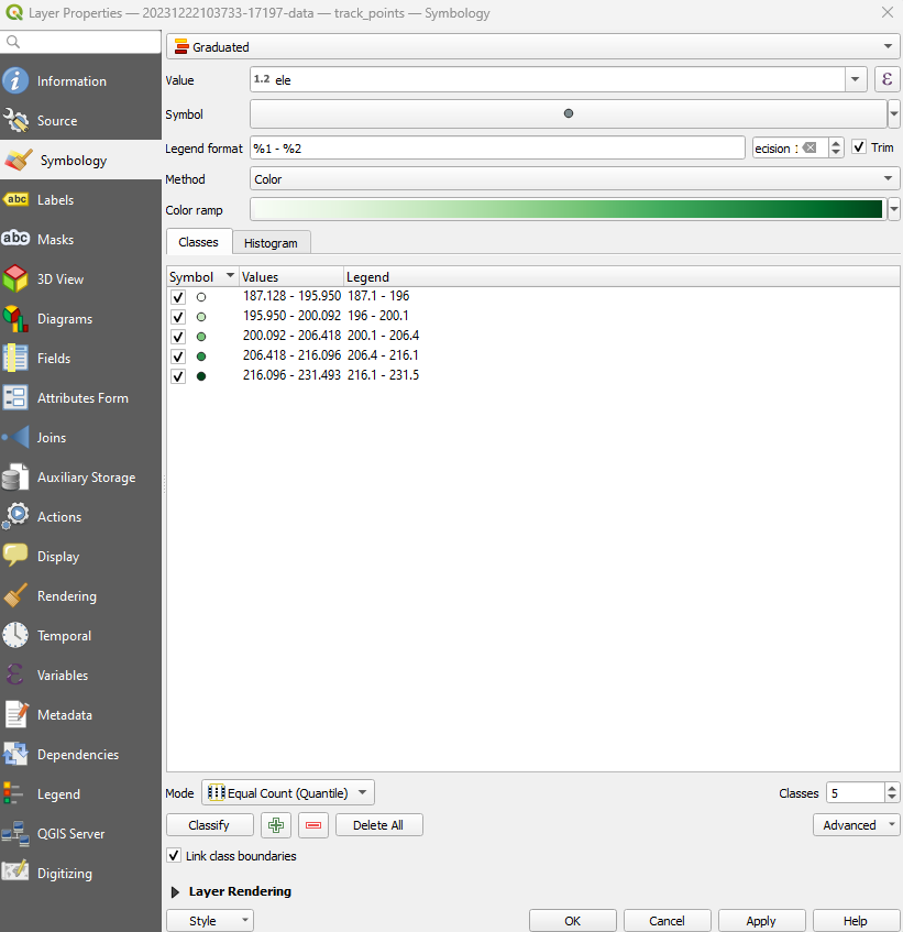
- Right-click on the gpx layer and select properties.
- Select Symbology from the Layer properties.
- Set value to “ele.”
- Set the number of classes to 5.
- Click Ok.

Creating topographic contours from elevation data
A topographic contour is a line on a map that represents points of equal elevation. That is, everything on the ground that lies on that line is the same elevation. Contours are often used to illustrate the shape and elevation of the terrain as an alternative way for the map viewer to understand the topography of an area on a two-dimensional map.
Converting a raster elevation layer to contours in QGIS involves using the “Contour” tool, which creates lines of equal elevation based on the input raster.
To create contours from the resulting raster file:
- Select Raster from the menu tools.
- Select Extraction.
- Select Contour.
- From the contour window, set contour interval to 8m.
- Set resulting contour file to your desired output name and location.
- Click Run.
